
An overview of 3D plant phenotyping methods
Currently there is quite a significant amount of hype regarding 3D reconstructions of plants. We have received a number of requests for our sensor and many people have ideas on how to measure plants in 3D or are asking us what is currently the best way and method to answer their question and application. The reason for the hype is that first the ‘sensor-to-plant’ concept is becoming increasingly more and more important. It is less expensive compared to conveyor based solutions and enables field phenotyping with higher throughput. In order to assess plants morphological information of a plant that is fixed, 3D plant phenotyping is the method of choice. Moreover, 3D plant phenotyping also allows researchers to gather plant architecture which is fundamental to improvement of traits such as light interception of plants. Lastly, many optical sensors that use spectral information such as hyperspectral or thermal imaging strongly depend on the inclination and distance of the plant organ, hence 3D information is needed to correct those signals.
To scan or not to scan…
There are many different principles on how to acquire plants in 3D and it is easy to get confused about the differences and advantages of all those sensors. For this reason, I decided to write this blog and give you an overview on the different methods and sensors for 3D plant phenotyping. I don´t want to go into deep technical discussions, but rather focus on the pros and cons of each principle for different applications in plant phenotyping.
I want to start with two brief substantial definition, which separates the sensors and their output into different groups
The first definition separates sensors into cameras and scanners:
A camera takes an image with two spatial dimensions (2D) within one shot. The result is a 2D matrix with values for each x-y pair. For cameras that measure depth the values in those 2D matrices typically store the distance from the sensor in this x-y value pair.
A scanner can only acquire a one dimensional line at a time. The result is therefore a vector with the corresponding height values. By moving the scanner over the scene and concatenating multiple vectors after each other you will receive the second spatial dimension.
The second definition categorizes the output of these sensors to be either a real 3D scene (point cloud or vertex mesh) or a 2D grey-scale depth map.
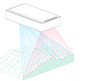
The resulting data for both cameras and scanners is often not a real 3D image but a 2D depth image with height as the values of the x-y-pairs (sometimes referred to as 2.5D). Each x-y- location in the image will just have one distance value. Therefore structures like overlaying leaves can’t be detected (see Fig. 1 you can’t see behind the objects in the image).
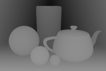
Fig. 1: Depth image of a stereo camera. The grey value of each pixel represents the distance from the camera. Objects behind the projected surface can’t be measured.
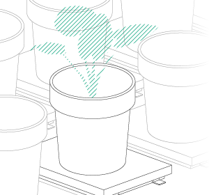
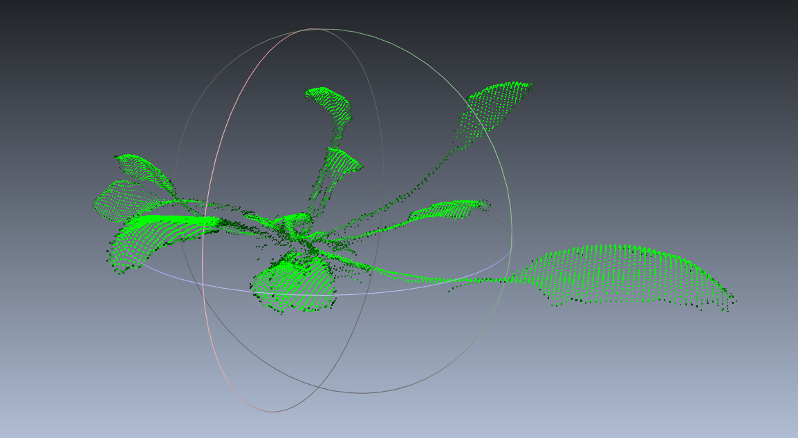
When using multiple angles that measure the whole scene, both concepts scanners and cameras can increase this 2.5D to a real 3D scene where overlaps can be detected. The data will then be a real 3D point cloud with x-y-z coordinates with an additional value such as colour stored for each of those triplets (see Fig. 2 that you can actually rotate and look at the plant from all dimensions).
Fig. 2: Full 3D scan of a cabbage plant measured with 2 laser scanners. Even overlapping leaves on the right side of the plant can be detected. Both scanners have been mounted on top of the plant with an angle. The scan is made without rotating or moving the plant.
After this short definitions let me continue to compare different methods for 3D plant phenotyping. I will describe the measurement principle for each method and show an illustration how it works. After this I will briefly compare pros and cons of each method.
LIDAR
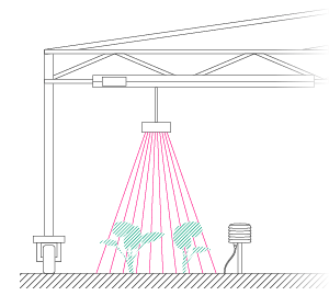
A LIDAR (Light Detection And Ranging) uses a combination of a detector and a laser and projects a small dot onto the object. This dot is moved at high velocity over the whole scene while the detector samples it. The detector measures the runtime of the reflection of the laser returning from the object. As the speed of light can be considered constant, the distance from each point to the detector can be calculated. The illustration in Fig. 3 shows how the laser dot is moved across the scene. The movement is often achieved by using one or multiple rotating mirrors. Modern LIDAR sensors can also use multiple lasers to increase imaging speed [1, 2].
(Side-Note: Ever got a speeding ticket? Maybe it was a LIDAR that caught you. Law enforcement use LIDAR to measure the distance of an approaching car. By measuring how much closer a car got between two consecutive measurements they can estimate the speed very accurately before you can even see them.)
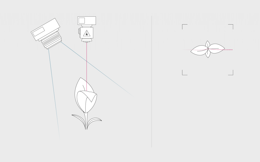
Fig. 3: LIDAR project a laser point over the whole image and measure the phase shift when the point is reflected back into the detector.
Pros
- Fast image acquisition: LIDAR is a very fast technology that allows scanning at high frequency (Scan rate of 25 – 90Hz). The laser dots are rotated via precision mirrors and can be moved at high velocity over the scene.
- Light independent: LIDAR uses its own light source and is therefore independent of ambient light conditions, measurements can also be performed at night.
- High scanning range: LIDAR can be used on large distances (2m – 100m) and also works from airborne vehicles (with lower depth resolution). Although, depth resolution might not be as accurate as other methods, the flexibility in range is outstanding.
Cons
- Poor X-Y resolution: Highest resolution of a LIDAR sensor is around 1 cm – 10cm, since the laser dot that is projected on plants is typically 2-8 mm meaning that fine structures, small plant organs, seedlings, ears, tillers, etc. can hardly be assessed. One important specification of a LIDAR is therefore the smallest detectable area (or laser footprint).
- Bad edge detection: 3D point clouds of edges of plant organs like leaves for instance are very blurry and need further processing. The reason for this unsharpened edges, is that the laser dot projected on the edge is partly reflected from the border of the leaf and the other part from some other parts in the background. Therefore, the returning signal or height information is an average of the two reflecting parts.
- Need for calibration: Its rotating mirrors are a source of errors since after some operational time mechanical parts might be deregulated, which requires recalibration. Various papers present calibration routines for different LIDAR models such as [16].
- Warm-Up time: It has been shown that the lasers used in LIDAR often require a warm-up time of up to 2.5 h. Within that time the output of depth information might not be stable. When using a LIDAR with multiple lasers warm up times for each laser can also differ and produce random noise in the depth map.
- Need for movement: Normally LIDAR is a scanner, and therefore the system requires a constant movement. As a consequence, the scanning of a single plant will take some time and hence movement of plants due to wind or other reasons reduces the quality of the 3D point cloud.
Laser Light Section
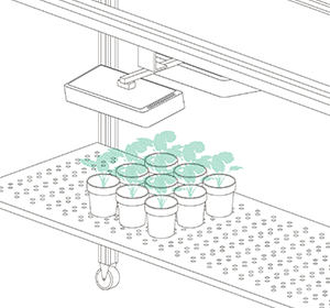
Similar to LIDAR, a laser light section scanner projects a laser on the object. Unlike LIDAR it’s not a point but a thin line instead. In contrast to LIDAR, not the runtime of the laser but its shift due to objects in the image is used (Fig. 4). The laser line is shifted by any object in the scene in function of the distance towards the sensor. Based on that shift the scanner can compute the distance of the object to the camera and create a depth profile. [11, 12]. Some examples for this technology can be found here.
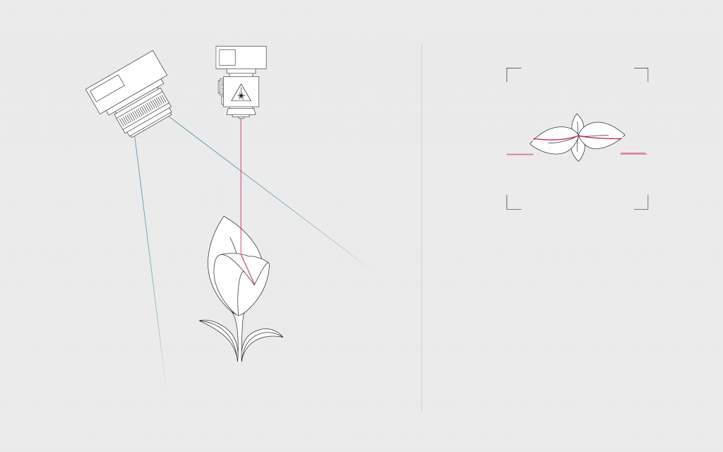
Fig. 4: A laser line is reflected on the object. The camera measures the reflectance and the shift in the image under a certain angle. A bigger angle produces a higher depth resolution. High imaging angles also increase shadow effects where the camera is ‘blind’ because the laser line is shaded.
Pros
- Fast image acquisition: Laser line scanners are fast meaning that they can measure (around 50Hz and more). Although, LIDAR may outperform them in speed they have a higher accuracy in all dimensions especially in the X-Y plane.
- Light Independent: Laser line scanners use their own light source and therefore are independent of ambient light conditions and work also without any surrounding light. In return the sensor is very susceptible to sunlight. However, some sensors such as PlantEye (linked) can handle even strong sunlight due to special filtering methods.
- High Precision: Laser line scanners can have a very high precision in all dimensions (up to 0.2mm) as the laser line and the camera can be very well calibrated and can even deliver a higher resolution than the chip sized using sub-pixel statistics.
- Robust Systems: The sensor does not have any moving parts. For this reason the sensor is very robust, needs only little maintenance or recalibration and can be used under harsh and remote conditions.
- Need for movement: As it is a scanner, the system requires a constant movement, so either the scanner moves over plants or plants are moved below the scanner. Therefore, the scanning of a single plant will take some time and hence movement of plants due to wind or other reasons reduces the quality of the 3D point cloud.
- Defined range: The scanner can be calibrated to a certain range (typically between 0.2m and 3m) and can only focus on the laser if it is within that range. This method allows very high precision but decreases flexibility.
Cons
- Need for movement: As it is a scanner, the system requires a constant movement, so either the scanner moves over plants or plants are moved below the scanner. Therefore, the scanning of a single plant will take some time and hence movement of plants due to wind or other reasons reduces the quality of the 3D point cloud.
- Defined range: The scanner can be calibrated to a certain range (typically between 0.2m and 3m) and can only focus on the laser if it is within that range. This method allows very high precision but decreases flexibility.
Structured Light
This method uses structured light instead of just one line. Multiple lines or defined light patterns are projected on the plant. The shift of the pattern depends on the distance from the sensor to the plant, from which you can compute depth information. The easiest way to imagine this concept is to think of a big man wearing a striped shirt. The pattern of the shirt will be bent. The bigger the bend, the bigger the tummy! A well-known example for the structured light principle is the Microsoft Kinect that projects an infrared pattern onto the object to assess the depth information of objects. [8-10]
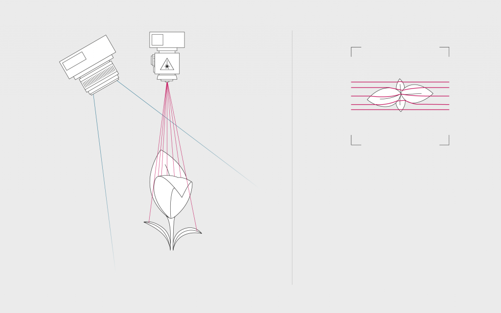
Fig. 5: a pattern is reflected on the object. The camera will measure the pattern and the shifts in the pattern to reconstruct the distance of the object in the scene. Often the projectors used for the pattern are working in the near infrared spectrum.
Pros
- Insensitive to movement: The system is a camera, which means that there is no movement required to assess the plants.
- Inexpensive System: Systems such as the Kinect are very cheap. This makes them attractive for simple applications where the sunlight problem (see below) can be avoided.
- Colour information: Sensors such as the Kinect combine structured light cameras and RGB cameras. The cameras can assess depth images and colour images at the same time. However, illumination can be a constraint when acquiring colour information over day.
Cons
- Susceptible to sunlight: The used IR patterns can be easily overexposed by sunlight or lighting systems for plants in greenhouses or climate chambers. Therefore the method is only suitable for screening at night or in closed imaging boxes.
- Poor x-y resolution: The current sensors only provide rudimentary X-Y resolution. One of the reasons is the limited resolution of Infra-Red Detectors that are used to measure the IR pattern (around 640×480 px).
- Poor depth resolution: The resolution of most structured light approach is not very high (typically around 3mm in 2m distance). Only high precision systems that are very close to the scanned object allow higher precision.
Stereo Vision
Stereo vision works in the same manner as our human vision, using two eyes to view the same scene. Analogously stereo vision uses two cameras, which are mounted next to each other (rule of thumb, the distance between the cameras should be around 10% of the distance between the plant and the cameras). Both cameras take an image of the same scene at same time. As shown in figure 1 the same object is at different positions on the two images since the perspective of the cameras is slightly different (A and B). The distance from the camera to that object can then be calculated based on the so-called disparity. The disparity is the “shift” of the object from left to right from one image to the other. Hence, an object close to the stereo setup will have a bigger disparity, compared to an object, which is further away [3-7].
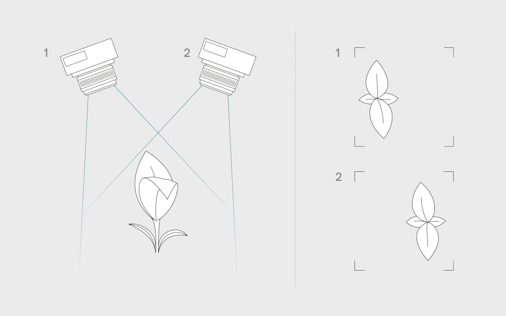
Fig. 6: Stereo vision uses two cameras to measure the same scene. As can be seen on the right, the same object will be in different locations in the two images. This shift is called disparity and can be used to calculate the distance from the camera of this object.
Pros
- Insensitive to movement: The system is a camera. That means that you acquire a 2D depth image without the need to move. Of course you need to move the sensor anyways if you want to screen multiple plants, but this one shot principle makes the system less susceptible to plant movement due to wind or other reasons.
- Inexpensive System: Industrial cameras are cheap and widely used. There are various cameras available on the market that are suitable for stereo reconstruction or already use a stereo concept.
- Colour information: The cameras can assess height information and colour at the same time. However, illumination can be a constraint when acquiring colour information over day.
Cons
- Susceptible to sunlight: A stereo setup does not bring its own light source (it can be extended with a flashlight or structural light approaches). Hence, results can be strongly susceptible to sunlight or the light sources used. The gathered colour information therefore needs to be calibrated.
- Poor Depth Resolution: The resolution in depth can be limited and is also depending on the structure of the objects, the local contrast as well as the angle of both cameras to each other.
- Computationally complex: The reconstruction of the 3D scene can be very complex as identical structures need to be detected in both images and aligned to compute the disparity. However, exploiting recent advances from GPU computing one can account for this.
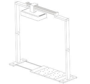
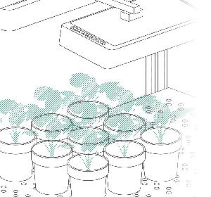
Space Carving
Space carving describes a multi-view 3D reconstruction algorithm. The same object is imaged from multiple angles. In each image the object of interest will be detected and a binary mask will be extracted. This binary mask is the projected shape of the object from a certain point of view. In the next step this mask is projected according to the angle of view it was measured with onto a fully filled cube and all parts that are not part of the shape will be carved away. With each additional image that is projected more and more volume of the cube will be carved away until only the real 3D object is left.
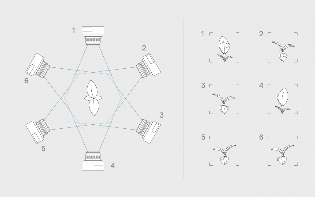
Fig. 4: Image acquisition for space carving. Multiple cameras are aligned around the object. The different perspectives will be merged into one full 3D point cloud of the object.
Pros
- Colour information: The cameras can assess depth information and colour at the same time.
- Complete Point clouds: Space carving can (when well implemented) produce very high quality, dense and complete point clouds. When the plant is imaged from all angles (at least 6 cameras are needed depending on the shape) you will have a full 3D model and not just a 2.5D depth image. Therefore, the effect of occlusion is reduced. Nevertheless, concave holes in the surface of the object that cannot by definition be detected by space carving as none of the projected images can show them properly.
- Fast Image acquisition: Space carving uses cameras. That means that you acquire the 2D input image relatively fast without the need to move the cameras. However, this requires that you have multiple cameras that measure the same object from different points of view. As an alternative the object can also be rotated to acquire multiple views with the disadvantage that movements (e.g. swinging after accelerating) of the object can strongly influence the 3D shape.
Cons
- Well-conditioned imaging boxes: Space carving often requires a clear imaging setup. A clear background and homogenous illumination are often needed to detect the binary masks that are computed before carving. As a lot of cameras need to look at the object from various angles it can only be used when there is a lot of space available.
- Expensive Setup: Multiple cameras or rotating devices are needed to reconstruction a 3D model with space carving. Therefore, the hardware setup of such systems can be expensive. Easily the carving process needs 6 or more images to create good results. Therefore 6 cameras would be needed or 6 images need to be recorded while turning the object. The later approach can become time consuming.
- Susceptible to movements: When the object moves during the acquisition the carving will remove points that are part of the object. For plants such as corn in particular this can lead to gaps or missing leaves in the point cloud.
- Computationally complex: The reconstruction of the 3D scene can be very complex. Each image must be projected onto the cube and carved out of the cube. Besides the computational power there is also high memory requirement to store all images and the data cube. The cube itself should be stored in a fast format (e.g. an Octree) as it needs to be completely read multiple times during the process. Recent advances from GPU computing can improve the reconstruction speed.
- Plant to Sensor Concept: To generate the needed input images, the plant needs to be accessible from all sides. In dense field rows this approach is not suitable. Space carving so far is mainly applied in closed imaging boxes. Therefore, the plant needs to be brought into those imaging boxes (either manually or by conveyors).
Other technologies
Aside from the technologies mentioned above several people deployed Time of Flight (ToF) cameras for plant phenotyping. ToF cameras use a near infrared emitter and measure the time it takes for the signal to be reflected calculated by the phase shift. Current disadvantages are their poor depth resolution (which is also depending on the colour of the reflecting surface) and that these sensors are not suitable to use under strong sunlight. Similar to stereo cameras ToF systems are also a camera and can – other than stereo – also be used with objects of low contrast. [13, 14]
A last 3D technology light field camera. These systems use conventional CCD cameras in combination with micro lenses to measure not only the position and intensity of the incoming light but also to calculate its origin. With this information the distance of the original object can be recalculated. Light-field cameras require very high resolution sensors with all consequences (expensive cameras and very expensive lens systems). First applications in life science have been done recently and show promising results. [15]
Conclusion
There is not the one 3D measurement method that solves all requirements, but one should rather choose the principle following the needs and the budget. LIDAR, laser line scanners and stereo vision have proven their performance and show most advantages for assessing plants. As all three originate from industry applications such as quality control or manufacturing, those sensors can be adapted and validated for the use in plant phenotyping. However, the biggest assets are their insusceptibility to sunlight. Laser line scanners have proven to be efficacious in field and greenhouse applications.
All single perspective plant phenotyping sensors described are imitated by occlusions (i.e. overlapping leaves that hide inner structures). Whenever a structure is covered and the sensor cannot “see” it, it will be not visible in the 3D image. Recent developments can combine multiple sensors (DualScan) and use this multi-view approach to improve the data quality. However, even with unlimited amount of sensors one can’t completely remove occlusion effects.
The complexity and also the limitations make clear that for every application there might be a special sensor required. So, if you are planning to use such tools in your phenotyping experiments you should consider to test them and to get a feeling about the advantages but also the limitations.
References
- Omasa, K.; Hosoi, F.; Konishi, A. 3D lidar imaging for detecting and understanding plant responses and canopy structure. J. Exp. Bot. 2007, 58, 881–898. [Google Scholar]
- Hosoi, F.; Omasa, K. Estimating vertical plant area density profile and growth parameters of a wheat canopy at different growth stages using three-dimensional portable lidar imaging. ISPRS J. Photogramm. Remote Sens. 2009, 64, 151–158. [Google Scholar]
- Biskup, B.; Scharr, H.; Schurr, U.; Rascher, U. A stereo imaging system for measuring structural parameters of plant canopies. Plant Cell Environ. 2007, 30, 1299–1308. [Google Scholar]
- Mizuno, S.; Noda, K.; Ezaki, N.; Takizawa, H.; Yamamoto, S. Detection of wilt by analyzing color and stereo vision data of plant. In Computer Vision/Computer Graphics Collaboration Techniques; Springer: Berlin/Heidelberg, Germany, 2007; pp. 400–411. [Google Scholar]
- Takizawa, H.; Ezaki, N.; Mizuno, S.; Yamamoto, S. Plant recognition by integrating color and range data obtained through stereo vision. JACIII 2005, 9, 630–636.
- Rovira-Más, F.; Zhang, Q.; Reid, J. Creation of three-dimensional crop maps based on aerial stereoimages. Eng. 2005, 90, 251–259. [Google Scholar]
- Jin, J.; Tang, L. Corn plant sensing using real-time stereo vision. Field Robot. 2009, 26, 591–608. [Google Scholar]
- Paulus, S.; Behmann, J.; Mahlein, A.-K.; Plümer, L.; Kuhlmann, H. Low-cost 3D systems: Suitable tools for plant phenotyping. Sensors 2014, 14, 3001–3018. [Google Scholar]
- Chéné, Y.; Rousseau, D.; Lucidarme, P.; Bertheloot, J.; Caffier, V.; Morel, P.; Belin, É.; Chapeau-Blondeau, F. On the use of depth camera for 3d phenotyping of entire plants. Comput. Electr. Agric. 2012, 82, 122–127. [Google Scholar]
- Azzari, G.; Goulden, M.L.; Rusu, R.B. Rapid characterization of vegetation structure with a microsoft kinect sensor. Sensors 2013, 13, 2384–2398. [Google Scholar]
- Dornbusch, T., Lorrain, S., Kuznetsov, D., Fortier, A., Liechti, R., Xenarios, I., & Fankhauser, C. (2012). Measuring the diurnal pattern of leaf hyponasty and growth in Arabidopsis–a novel phenotyping approach using laser scanning.Functional Plant Biology, 39(11), 860-869. [Google Scholar]
- Kjær, K. H. Non-invasive plant growth measurements for detection of blue-light dose response of stem elongation in Chrysanthemum morifolium. In 7th International Symposium on Light in Horticultural systems. [Google Scholar]
- Kraft, M.; Salomão de Freitas, N.; Munack, A. Test of a 3d time of flight camera for shape measurements of plants. Proceedings of the CIGR Workshop on Image Analysis in Agriculture, Anchorage, AK, USA, 3–8 May 2010; pp. 108–115. [Google Scholar]
- Klose, R.; Penlington, J.; Ruckelshausen, A. Usability study of 3D time-of-flight cameras for automatic plant phenotyping. Bornimer Agrartech. Ber. 2009, 69, 93–105 [Google Scholar]
- Bishop, T. E., & Favaro, P. (2012). The light field camera: Extended depth of field, aliasing, and superresolution. Pattern Analysis and Machine Intelligence, IEEE Transactions on, 34(5), 972-986. [Google Scholar]
- Lichti, D. D. (2007). Error modelling, calibration and analysis of an AM–CW terrestrial laser scanner system. ISPRS Journal of Photogrammetry and Remote Sensing, 61(5), 307-324. [Google Scholar]